WONA_IN_IT

안녕하세요.

저번 sklearn LDA 토픽 모델링 게시물에 이어서 이번에는 선정한 토픽에 대해

기간별로 어떻게 변화하는지를 확인해 보도록 하겠습니다.

데이터 준비

데이터는 저번 게시물에서 사용한 데이터를 사용하겠습니다.

- 데이터: 공공데이터 포탈의 '공정거래위원회_소비자 민원학습데이터 처리기관별 소비자 상담내역' 

링크 들어가셔서

'공정거래위원회_소비자 민원학습데이터 처리기관별 소비자 상담내역_20211227.csv' 

파일을 다운받아 주세요.

import pandas as pd
df = pd.read_csv('공정거래위원회_소비자 민원학습데이터 처리기관별 소비자 상담내역_20211227.csv',encoding='cp949')
print(df.head())
print(df.shape)

이 데이터에서 날짜 데이터도 있고 기타 데이터도 많지만,

토픽 모델링은 사건 제목을 가지고 해보도록 하겠습니다.

#토픽 토크나이저를 위해 필요한 부분 (사건제목) 추출
contents= df['사건제목(ACCIDENT_TITLE)']
contents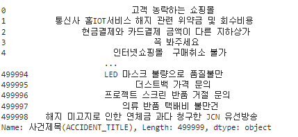

텍스트 토크나이징 및 카운트 벡터화

from konlpy.tag import Okt
from sklearn.feature_extraction.text import CountVectorizer
###형태소 분석###
okt = Okt()
def tokenizer(text):
    #명사 추출, 2글자 이상 단어 추출
    return [ word for word in okt.nouns(text) if len(word)>1]
Count_vector = CountVectorizer(tokenizer=tokenizer,
                              max_df = 0.5,
                              min_df = 5,
                              max_features = 2000)

%time minwon_cv = Count_vector.fit_transform(contents) 
print(minwon_cv[:5])
print(minwon_cv.shape)

이번에는 토픽 수를 선정해 보겠습니다.

sklearn를 사용하는 경우, 혼란도만 제공하고 있는데, tmtoolkit을 사용하면 응집도도 구할 수 있습니다.

토픽에 따른 혼란도, 응집도 및 토픽 내용을 print해주는 함수를 하나 만들어 실행해 보도록 하겠습니다.토픽 수는 3에서 10까지 늘려 값을 확인해 보겠습니다.

import numpy as np
import matplotlib.pyplot as plt
from sklearn.decomposition import LatentDirichletAllocation
from tmtoolkit.topicmod.evaluate import metric_coherence_gensim

# 토픽별 단어를 보여주는 함수
def print_top_words(model, feature_names, n_top_words):
    for topic_idx, topic in enumerate(model.components_):
        print("토픽 #%d: " % topic_idx, end='')
        print(", ".join([feature_names[i]
                        for i in topic.argsort()[:-n_top_words -1:-1]]))
                        
# 혼란도 및 응집도 구하는 함수
def calc_pv_coherence(countVector,vocab, start=5, end=30, max_iter=10,topic_wp=0.1, doc_tp=1.0):
    num = []
    per_value = []
    cor_value = []
    for i in range(start,end+1):
        lda = LatentDirichletAllocation(n_components=i,max_iter=max_iter,
                                       topic_word_prior=topic_wp,
                                       doc_topic_prior=doc_tp,
                                       learning_method='batch', n_jobs=-1,
                                       random_state=0)
        lda.fit(countVector)
        num.append(i)
        pv = lda.perplexity(countVector)
        per_value.append(pv)
        coherence_score = metric_coherence_gensim(measure='u_mass',
                                                  top_n=10,
                                                  topic_word_distrib=lda.components_,
                                                 dtm=countVector,
                                                 vocab=vocab,
                                                 texts=None)
        cor_value.append(np.mean(coherence_score))
        
        print(f'토픽 수: {i}, 혼란도: {pv:0.4f}, 응집도:{np.mean(coherence_score):0.4f}')
        print_top_words(lda, vocab,10)
    
    plt.plot(num,per_value,'g-')
    plt.xlabel("topic_num")
    plt.ylabel("perplexity")
    plt.show()
    
    plt.plot(num,cor_value,'r--')
    plt.xlabel("topic_num")
    plt.ylabel("coherence_score")
    plt.show()
    return per_value,cor_value

per_values, cor_values = calc_pv_coherence(minwon_cv,names,start=3,end=10)

이렇게 토픽 갯수별 토픽 단어들이 나오고,

토픽별 혼란도, 응집도를 확인했을 때 최적의 토픽 수는 4 로 보입니다.

선정된 토픽 갯수로 LDA 토픽 모델링 하기

sklearn LDA를 사용해서 4개의 토픽을 가지고 있는 모델을 만들어 보겠습니다.

from sklearn.decomposition import LatentDirichletAllocation
lda = LatentDirichletAllocation(n_components=4,
                               n_jobs= -1,
                               random_state=0,
                               max_iter=10,
                                topic_word_prior=0.1,
                               doc_topic_prior=1.0,
                               learning_method='batch',
                               )

minwon_topics = lda.fit_transform(minwon_cv)

토픽 모델링 한 결과는 아래와 같습니다. 각 토픽별로 상위 20개 단어를 보도록 하겠습니다.

print_top_words(lda, Count_vector.get_feature_names_out(),20)

트렌드 확인하기

이제 이 민원 토픽들을 가지고 시간별로 어떤 종류의 토픽이 많이 나왔는지 확인하기 위한 트렌드 분석을 진행해 보겠습니다.

날짜 데이터는 '등록일자(RCPT_YMD)' 컬럼에 있습니다. 

행이 5만개가 되기 때문에 날짜를 월단위까지만 자른 데이터를 토픽 분포 데이터와 합치도록 하겠습니다.

from sklearn.feature_extraction.text import CountVectorizer
trend_data = pd.DataFrame(minwon_topics,columns=['토픽'+str(i) for i in range(1,5)])
trend_data = pd.concat([trend_data,df['등록일자(RCPT_YMD)'].map(lambda x:x[:7])], axis=1)
trend_data.head()

이후 groupby를 사용하여 월 단위로 토픽의 평균을 구해보겠습니다.

#월별 평균 구하기
trend = trend_data.groupby(['등록일자(RCPT_YMD)']).mean()
trend.head()

이제 월별로 토픽 비중이 어떻게 변했는지 확인하기 위해 matplotlib을 사용하여 그래프를 그려 보도록 하겠습니다.

matplotlib의 AutoDateLocator를 사용하여 x축은 6개월 단위로 눈금 및 값을 표시해서 보여주도록 하겠습니다.

import matplotlib
import matplotlib.pyplot as plt
from matplotlib import font_manager,rc
from matplotlib.dates import AutoDateLocator,MonthLocator
# 한글 폰트 설정
font_location = 'C:/Windows/Fonts/MALGUNSL.TTF' #맑은고딕
font_name = font_manager.FontProperties(fname=font_location).get_name()
rc('font',family=font_name)
#날짜설정
locator = AutoDateLocator()
locator.intervald['MONTHLY'] = [6]

print_top_words(lda, Count_vector.get_feature_names_out(),20)

fig,axes = plt.subplots(2,2,figsize=(10,10))
for col,ax in zip(trend.columns.tolist(),axes.ravel()):
    ax.set_title(col)
    ax.xaxis.set_major_locator(locator)
    ax.axes.xaxis.set_visible(True)
    
    ax.plot(trend[col])

plt.show()

4개의 토픽에서 토픽별로 시간에 따라 분포가 어떻게 변화했는지 확인할 수 있습니다.

각 토픽 주제는 대략적으로

토픽 1: 피해 상담 문의

토픽2: 환불 및 반품 문의

토픽3: 수리 및 보상 문의

토픽4: 계약 해지 문의 

이렇게 볼 수 있을 것 같습니다.

토픽1 은 최근에 급격히 비중이 늘어났고, 토픽 3번은 시간에 따라 비중이 줄어들고 있고, 토픽 4번은 후반부에 비중이 늘어남을 확인할 수 있습니다.

 참고자료

1. 도서 - 파이썬 텍스트 마이닝 완벽 가이드(위키북스)

2.  https://scikit-learn.org/stable/modules/generated/sklearn.decomposition.LatentDirichletAllocation.html

3. https://matplotlib.org/stable/api/dates_api.html

https://www.data.go.kr/data/15098351/fileData.do#tab-layer-file

import pandas as pd
df = pd.read_csv('공정거래위원회_소비자 민원학습데이터 처리기관별 소비자 상담내역_20211227.csv',encoding='cp949')
print(df.head())
print(df.shape)

#토픽 토크나이저를 위해 필요한 부분 (사건제목) 추출
contents= df['사건제목(ACCIDENT_TITLE)']
contents

#카테고리 확인
df.groupby('처리결과명(PRCS_RESULT_NAME)').count()

print(len(df.groupby('처리결과명(PRCS_RESULT_NAME)').count()))

27

​

총 27개의 카테고리가 있습니다.

텍스트 토크나이징 및 카운트 벡터화

from konlpy.tag import Okt
from sklearn.feature_extraction.text import CountVectorizer
###형태소 분석###
okt = Okt()
def tokenizer(text):
    #명사 추출, 2글자 이상 단어 추출
    return [ word for word in okt.nouns(text) if len(word)>1]
Count_vector = CountVectorizer(tokenizer=tokenizer,
                              max_df = 0.5,
                              min_df = 5,
                              max_features = 2000)

%time minwon_cv = Count_vector.fit_transform(contents) 
print(minwon_cv[:5])
print(minwon_cv.shape)

이번에는 토픽 수를 선정해 보겠습니다.

sklearn의 경우, 혼란도만 제공하고 있는데, tmtoolkit을 사용하면 응집도도 구할 수 있습니다.

​

tmtoolkit 설치는 아래의 명령어를 입력하여 터미널에서 설치해 주시면 됩니다.

pip install --user tmtoolkit

sklearn에서 LDA는 sklearn.decomposition.LatentDirichletAllocation 을 사용하여 구할 수 있습니다.

sklearn LDA의 n_components는 추출할 토픽의 수를 의미하고,

max_iter는 알고리즘의 최대 반복 횟수(gensim의 passes라고 생각하면 됩니다.),

topic_word_prior은 베타값(토픽의 사전 단어분포),

doc_topic_prior은 알파값(문서의 사전 토픽분포),

learning_method는 학습방법으로 online과 batch가 있습니다.

n_jobs는 모델 사용시 사용하는 프로세서의 수를 의미하며 -1로 설정하면 모든 프로세서를 사용할 수 있습니다.

​

이번에는 max_iter를 10으로 설정하고,

topic_word_prior와 doc_topic_prior은 아래의 논문

https://www.ncbi.nlm.nih.gov/pmc/articles/PMC387300/

을 참고하여 각각 0.1, 1.0으로 설정해 보도록 하겠습니다.

random_state는 0으로 설정해준 뒤,

n_components는 5부터 30까지의 값을 넣어 실행한 뒤,

혼란도, 응집도 값을 각각 구해 matplotlib으로 시각화 해보도록 하겠습니다.

​

혼란도는 sklearn LDA 모형의 .perplexity로 값을 구하고,

응집도는 tmtoolkit.topicmod.evaluate.metric.coherence_gensim을 사용하여 구하도록 하겠습니다.

coherence score에서 measure은 'u_mass'를 사용하였습니다.

import numpy as np
import matplotlib.pyplot as plt
from sklearn.decomposition import LatentDirichletAllocation
from tmtoolkit.topicmod.evaluate import metric_coherence_gensim
def calc_pv_coherence(countVector,vocab, start=5, end=30, max_iter=10,topic_wp=0.1, doc_tp=1.0):
    num = []
    per_value = []
    cor_value = []
    for i in range(start,end+1):
        lda = LatentDirichletAllocation(n_components=i,max_iter=max_iter,
                                       topic_word_prior=topic_wp,
                                       doc_topic_prior=doc_tp,
                                       learning_method='batch', n_jobs=-1,
                                       random_state=0)
        lda.fit(countVector)
        num.append(i)
        pv = lda.perplexity(countVector)
        per_value.append(pv)
        coherence_score = metric_coherence_gensim(measure='u_mass',
                                                  top_n=10,
                                                  topic_word_distrib=lda.components_,
                                                 dtm=countVector,
                                                 vocab=vocab,
                                                 texts=None)
        cor_value.append(np.mean(coherence_score))
        
        print(f'토픽 수: {i}, 혼란도: {pv:0.4f}, 응집도:{np.mean(coherence_score):0.4f}')
    
    plt.plot(num,per_value,'g-')
    plt.xlabel("토픽 수:")
    plt.ylabel("혼란도: ")
    plt.show()
    
    plt.plot(num,cor_value,'r--')
    plt.xlabel("토픽 수:")
    plt.ylabel("응집도: ")
    plt.show()
    return per_value,cor_value

함수를 이렇게 만들고 아래와 같이 호출해 줍니다.

per_values, cor_values = calc_pv_coherence(minwon_cv,Count_vector.get_feature_names_out(),start=5,end=30)

결정된 토픽 수로 토픽 모델링 하기

lda = LatentDirichletAllocation(n_components=29,
                               n_jobs= -1,
                               random_state=0,
                               max_iter=10,
                                topic_word_prior=0.1,
                               doc_topic_prior=1.0,
                               learning_method='batch')

%time minwon_topics = lda.fit_transform(minwon_cv)

토픽 수 29로 LDA모델을 만들고 fit한 후 토픽을 뽑아보면,

for topic_idx, topic in enumerate(lda.components_):
    print("토픽 #%d: " % topic_idx, end='')
    print(", ".join([Count_vector.get_feature_names_out()[i] for i in topic.argsort()[:10]]))

for topic_idx, topic in enumerate(lda.components_):
    print("토픽 #%d: " % topic_idx, end='')
    print(", ".join([Count_vector.get_feature_names_out()[i] for i in topic.argsort()[:-11:-1]]))

참고자료

1. 도서 - 파이썬 텍스트 마이닝 완벽 가이드(위키북스)

2. https://scikit-learn.org/stable/modules/generated/sklearn.decomposition.LatentDirichletAllocation.html

3. https://alvinntnu.github.io/NTNU_ENC2045_LECTURES/nlp/topic-modeling-naive.html#additional-notes

안녕하세요.

이번에는 한국어 데이터셋을 가지고 gensim을 사용한 LDA 토픽 모델링 실습을 해보도록 하겠습니다.

데이터 준비

테이터셋으로 '청와대 국민청원' 에 만료된 청원 데이터를 사용하도록 하겠습니다.

아래 사이트 접속 후 

https://github.com/akngs/petitions

petition_sampled.csv 를 클릭하여 다운받아 주세요.

전체 데이터는 데이터 용량이 커서 샘플 데이터를 사용하겠습니다.

파일 불러오기

다운받은 파일중 5개만 예시로 출력해보겠습니다.

import pandas as pd
df = pd.read_csv('petition_sampled.csv')
df.head()

데이터는 위와 같이 구성되어 있는 것을 확인할 수 있습니다.

여기서 실습에서는 청원 내용을 가지고 토픽 모델링을 해보도록 하겠습니다.

때문에 content컬럼만 따로 뽑아줍니다.

contents = df['content']
contents

또한 원본 데이터에 카테고리 항목이 있는데 

데이터가 몇 개의 카테고리가 있는지도 한번 확인해 보겠습니다.

groupby를 사용하여 카테고리가 몇 개 있는지 확인해 보겠습니다.

len(df.groupby('category').votes.sum())

이렇게 17개의 카테고리가 있는 것을 확인할 수 있습니다.

참고로 가장 많은 votes 수의 카테고리는 '인권/성평등' 카테고리임을 확인할 수있습니다.

 토픽 모델링을 위한 텍스트 토큰화(형태소분석)하기

여기서는 Gensim을 사용하여 LDA 토픽 모델링을 해 볼 건데요,

gensim을 사용하면 혼란도와 토픽 응집도를 간단하게 구할 수 있어 많이 사용됩니다.

pip install gensim

을 터미널에 입력하여 설치할 수 있습니다.

gensim은 입력값으로 텍스트를 그대로 입력하는 것이 아닌 토큰화된 결과를 입력값으로 사용하므로

청원 내용을 형태소 분석을 통해 토큰화 해보도록 하겠습니다.

형태소 분석으로는 konlpy의 Okt를 사용하여 분석해 보겠습니다. 

단어 중 '명사' 및 2글자 이상의 단어만 추출해 보도록 하겠습니다.

from konlpy.tag import Okt
###형태소 분석###
okt = Okt()
def analysis_pos(text):
    morphs = okt.pos(text,stem=True)

    words = []
    #명사 추출, 2글자 이상 단어 추출
    for word, pos in morphs:
        if pos == 'Noun':
            if len(word) > 1:
                words.append(word)
    return words

texts = [analysis_pos(news) for news in contents]

이렇게 함수를 만들어 texts 변수 안에 토큰화한 텍스트를 저장하였습니다.

토큰화 된 텍스트로 gensim Dictionary 만들기

gensim LDA에서 id2word에 사용하기 위해 토큰화된 텍스트로 사전을 만들어 보겠습니다.

from gensim.corpora.dictionary import Dictionary
# 형태소 분석으로 토큰화 후 dictionary 생성
dictionary = Dictionary(texts)
print("#문서에 있는 단어 수: %d개"%len(dictionary))

문서에 있는 단어 수가 3만개가 넘는데요,

이를 filter_extremes를 사용해 단어를 2000개까지 설정하고 5개 미만으로 나온 단어는 제외, 전체 50% 이상으로 많이 나오는 단어들도 제외를 해보도록 하겠습니다.

keep_n 으로 단어 갯수를 설정하고, no_below로 일정 횟수 미만으로 나온 단어는 제외, no_above로 일정 비율 이상으로 나오는 단어들도 제외하도록 설정할 수 있습니다.

물론 다른 비율 또는 횟수, 갯수로 바꿔서 필터링 할 수 도 있습니다.

# 너무 많은 단어나 너무 적은 단어를 제외하고, 단어 빈도순으로 정리
dictionary.filter_extremes(keep_n=2000, no_below=5, no_above=0.5)
print("#너무 많은 단어 및 적은 단어를 제외하고 문서에 남아 있는 단어 수: %d개"%len(dictionary))

카운트벡터로 변환하기

gensim LDA 에 사용하기 위한 corpus를 생성하려면 doc2bow를 사용하여 카운트 벡터로 변환하여야 합니다.

gensim에서는 토큰화 된 결과를 texts라 하고 이것을 카운트 벡터로 변환한 것을 corpus라고 합니다.

# 카운트 벡터로 변환
corpus = [dictionary.doc2bow(text) for text in texts]
print("#최종적으로 문서에 있는 단어 수: %d개"%len(dictionary))
print("#카운트 벡터 수: %d개"%len(corpus))

Gensim LDA 모델 생성

gensim의 LdaModel을 사용해서 LDA 모델링을 수행할 수 있습니다.

num_topics은 토픽의 수를, passes는 말뭉치 전체를 학습하는 횟수, corpus는 토큰화한 값들을 카운트 벡터화 한것, id2word는 위에서 만든 dictionary를 입력하면 됩니다.

우선 원본 데이터가 총 17개의 카테고리를 가지고 있으므로,

num_topics를 17로 설정하여 모델링을 수행해 보도록 하겠습니다.

from gensim.models import LdaModel
num_topics = 17
passes = 5
model = LdaModel(corpus=corpus,id2word=dictionary,\
    passes=passes, num_topics=num_topics,\
        random_state=7)

그 후 모델링 한 결과를 각 토픽당 10개의 단어씩 뽑아서 보도록 하겠습니다.

model.print_topics(num_words=10)

pyLDAvis를 사용한 시각화

위의 모델링 결과를 한눈에 보기 쉽게 pyLDAvis를 사용하여 시각화할 수 있습니다.

설치는 pip install pyLDAvis 로 설치 가능합니다.

import pyLDAvis
import pyLDAvis.gensim_models as gensimvis
pyLDAvis.enable_notebook()

#LDA모형 시각화
lda_visual= gensimvis.prepare(model,corpus,dictionary)
pyLDAvis.display(lda_visual)

최적의 토픽 수 선정하기

원본이 17개 카테고리여서 num_topics를 17로 설정했지만 실제 분석시에는 카테고리조차 없는 데이터들도 있을 것입니다. 

또한 위의 결과도 최적의 토픽 개수를 설정한 것인지 알 수 없으므로 혼란도와 토픽응집도를 구해서 살펴보도록 하겠습니다.

gensim에서 .log_perplexity를 사용하면 혼란도를, CoherenceModel로 토픽응집도를 간편히 구할 수 있습니다.

여기서는 혼란도와 토픽 응집도를 구하는 함수를 만들고

for문을 사용하여 토픽 갯수당 각각의 혼란도, 응집도를 구해 그래프로 시각화 후 최적화를 진행해보겠습니다.

import matplotlib.pyplot as plt
from gensim.models import CoherenceModel
def coherences(corpus, dictionary, start=6,end=15):
    iter_num=[]
    per_value=[]
    coh_value=[]
    for i in range(start, end+1):
        model = LdaModel(corpus=corpus, id2word=dictionary,
                        chunksize=1000, num_topics=i,
                        random_state=7)
        iter_num.append(i)
        pv = model.log_perplexity(corpus)
        per_value.append(pv)
        CM = CoherenceModel(model=model, corpus=corpus, coherence='u_mass')
        coherence_value = CM.get_coherence()
        coh_value.append(coherence_value)
        print(f'토픽 수: {i}, 혼란도:{pv:0.3f}, 응집도: {coherence_value:0.3f}')
        
    plt.plot(iter_num,per_value,'g-')
    plt.xlabel("num_topics")
    plt.ylabel("perplexity")
    plt.show()
        
    plt.plot(iter_num, coh_value,'r--')
    plt.xlabel("num_topics")
    plt.ylabel("coherence")
    plt.show()

start는 토픽의 시작 갯수를, end는 마지막으로 구할 토픽 갯수입니다.

간단히 말해 for문의 시작과 끝을 설정한다고 볼 수 있습니다.

여기서는 토픽 5개~20개까지로 설정했을 때 각각의 혼란도, 토픽 응집도를 구해 보겠습니다.

coherences(corpus, dictionary, start=5,end=20)

혼란도는 낮을 수록 좋고 토픽 응집도는 0에 가까울수록 좋습니다.

위의 그래프를 보면 혼란도가 가장 낮게 나타난 곳은 17개이고, 토픽 응집도가 가장 0에 가까운 곳은 6개로

차이가 있음을 알 수 있습니다.

최적화가 쉽지 않아보이지만 둘 중 더 토픽을 잘 나타내는 것으로 최종 선택을 할 수 있겠습니다.

혼란도가 가장 낮은 토픽 17개로는 이미 전에 모델링을 실행해 보았으니,

이번에는 응집도가 가장 높은 토픽 6개로 모델링을 해보도록 하겠습니다.

num_topics = 6
passes = 5
model2 = LdaModel(corpus=corpus,id2word=dictionary,\
    passes=passes, num_topics=num_topics,\
        random_state=7)
        
model2.print_topics(num_words=10)

#LDA모형 시각화
lda_visual2= gensimvis.prepare(model2,corpus,dictionary)
pyLDAvis.display(lda_visual2)

이 둘 중에 또는 모델을 조정하여 최종적으로 토픽 수를 정할 수 있겠습니다.

코드 파일

참고자료

1. 책- 파이썬 텍스트 마이닝 완벽 가이드(위키북스)

2. https://radimrehurek.com/gensim/models/coherencemodel.html